Installation
Pure Python implementation of bayesian global optimization with gaussian processes.
- PyPI (pip):
1
$ pip install bayesian-optimization
- Conda from conda-forge channel:This is a constrained global optimization package built upon bayesian inference and gaussian process, that attempts to find the maximum value of an unknown function in as few iterations as possible. This technique is particularly suited for optimization of high cost functions, situations where the balance between exploration and exploitation is important.
1
$ conda install -c conda-forge bayesian-optimization
Basic Usage
1 | from sklearn.datasets import make_classification |
Visualization
Target Function
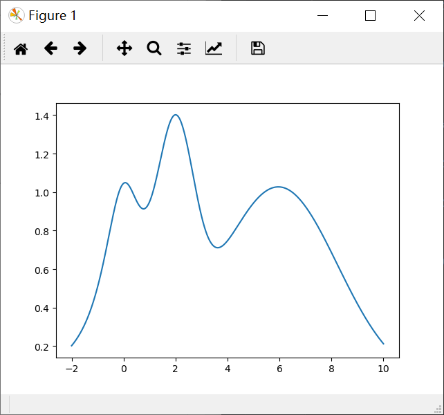
Lets create a target 1-D function with multiple local maxima to test and visualize how the BayesianOptimization package works. The target function we will try to maximize is the following:
$f(x)=e^{-(x-2)^2}+e^{-\frac{(x-6)^2}{10}}+\frac{1}{x^2+1}$
its maximum is at $x = 2$ and we will restrict the interval of interest to $x \in (-2, 10)$.
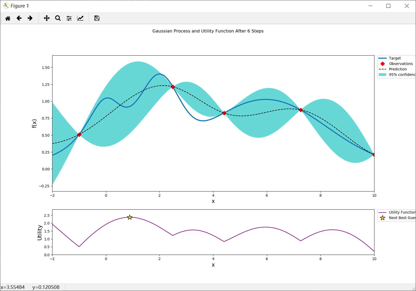
Notice that, in practice, this function is unknown, the only information we have is obtained by sequentialy probing it at different points. Bayesian Optimization works by contructing a posterior distribution of functions that best fit the data observed and chosing the next probing point by balancing exploration and exploitation.
1 | from bayes_opt import BayesianOptimization |
Stopping
After just a few points the algorithm was able to get pretty close to the true maximum. It is important to notice that the trade off between exploration (exploring the parameter space) and exploitation (probing points near the current known maximum) is fundamental to a succesful bayesian optimization procedure. The utility function being used here (Upper Confidence Bound - UCB) has a free parameter $\kappa$ that allows the user to make the algorithm more or less conservative. Additionally, the larger the initial set of random points explored, the less likely the algorithm is to get stuck in local minima due to being too conservative.
1 | | iter | target | x | |
Exploitation vs Exploration
Target function
1 | np.random.seed(42) |
Utility function for plotting
1 | def plot_bo(f, bo): |
Acquisition Function
Upper Confidence Bound (UCB)
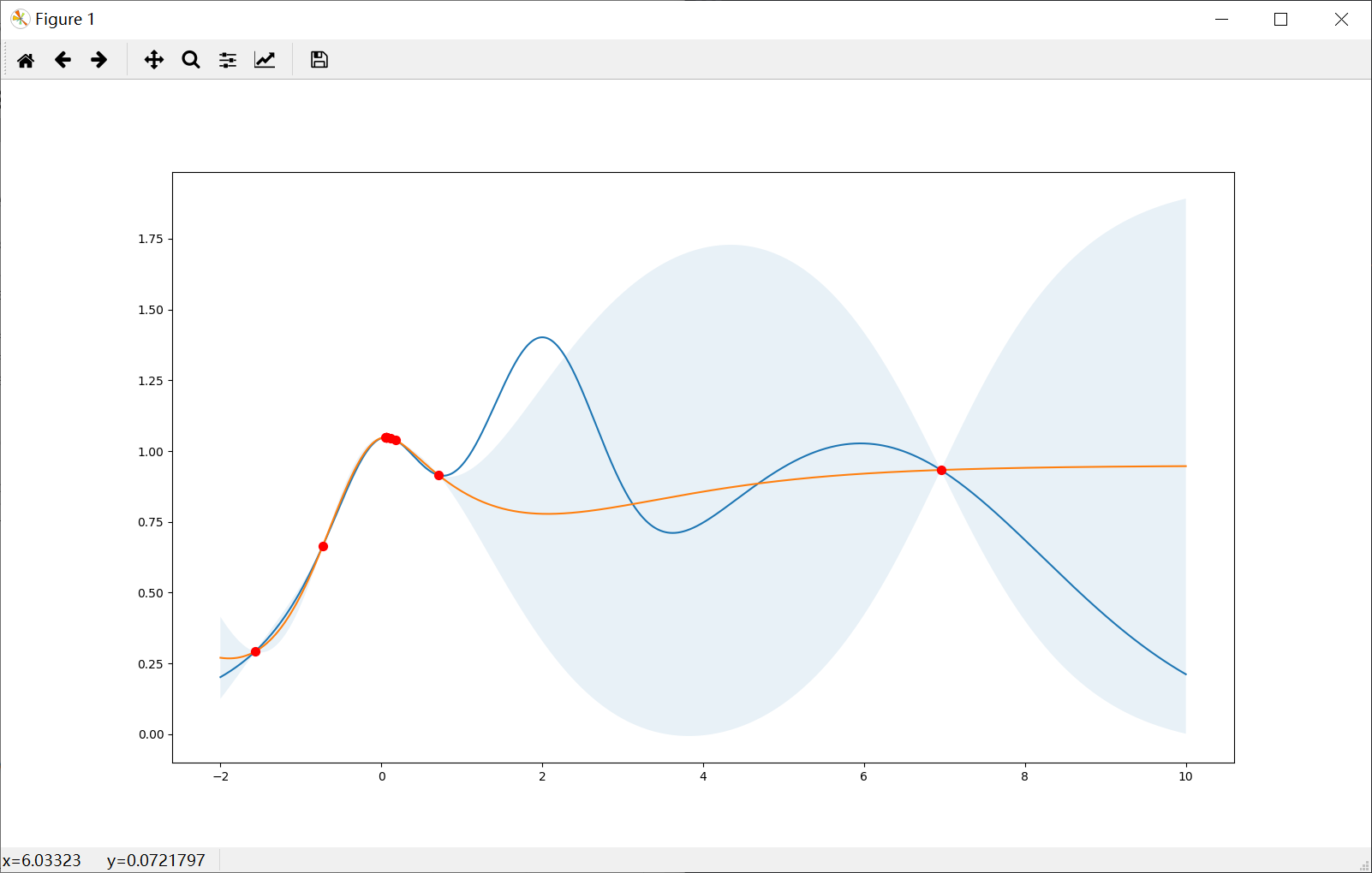
Prefer exploitation (kappa=0.1)
Note that most points are around the peak(s).
1 | bo = BayesianOptimization( |
Prefer exploration (kappa=10)
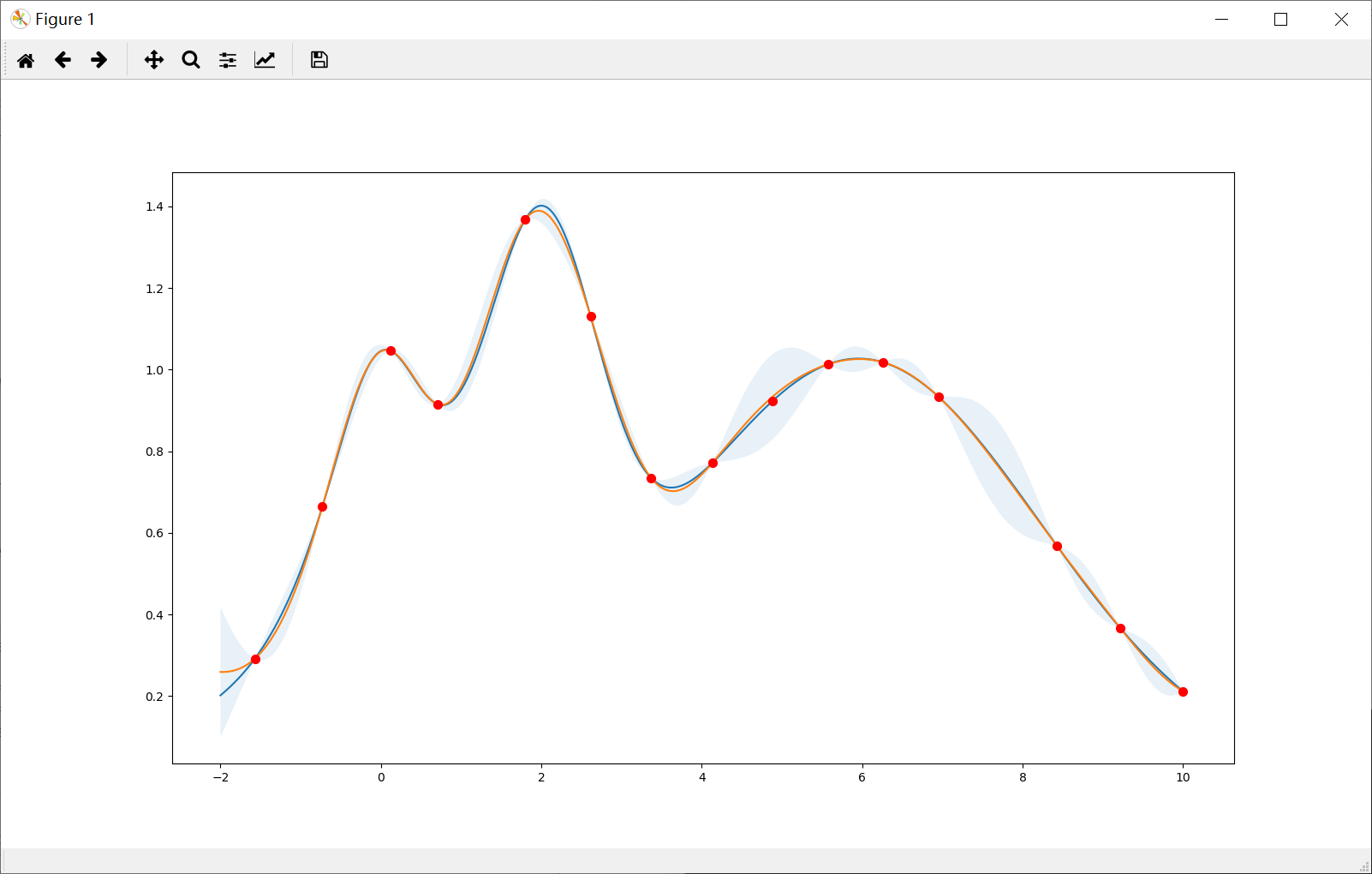
Note that the points are more spread out across the whole range.
1 | bo = BayesianOptimization( |
Expected Improvement (EI)
Prefer exploitation (xi=1e-4)
Note that most points are around the peak(s).
1 | bo = BayesianOptimization( |
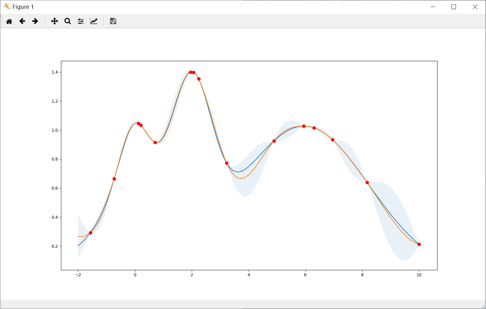
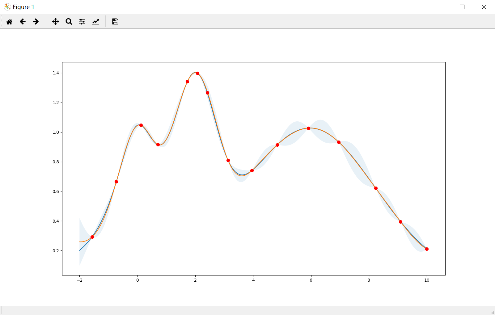
Prefer exploration (xi=1e-1)
Note that the points are more spread out across the whole range.
1 | bo = BayesianOptimization( |
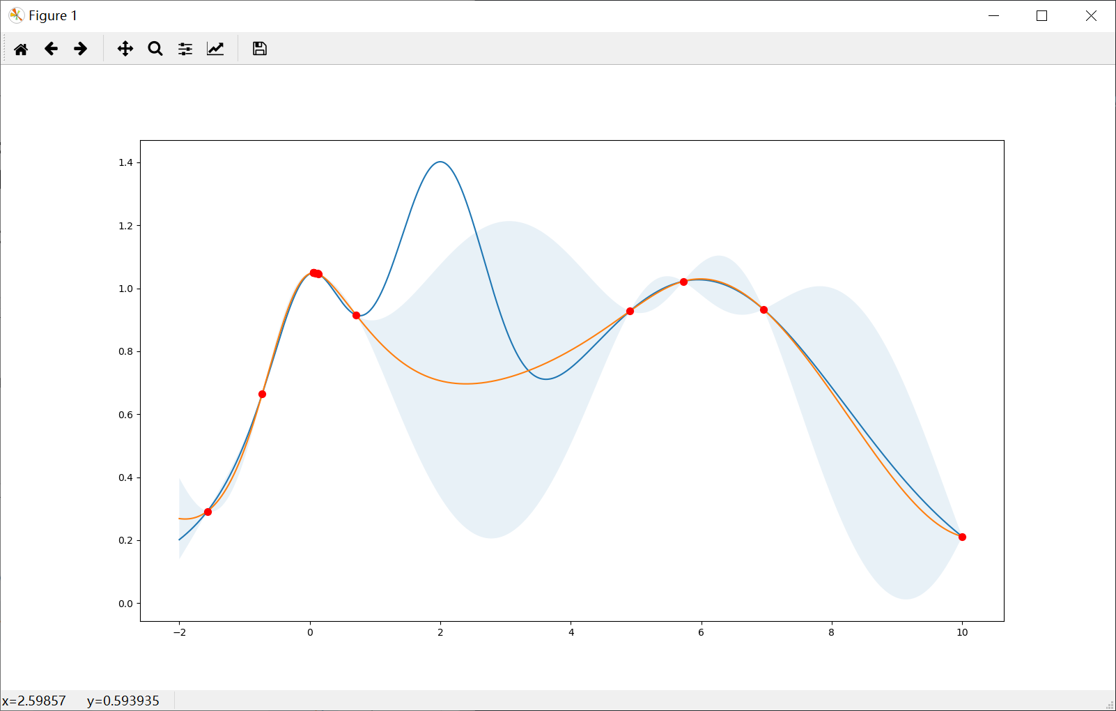
Probability of Improvement (POI)
Prefer exploitation (xi=1e-4)
Note that most points are around the peak(s).
1 | bo = BayesianOptimization( |
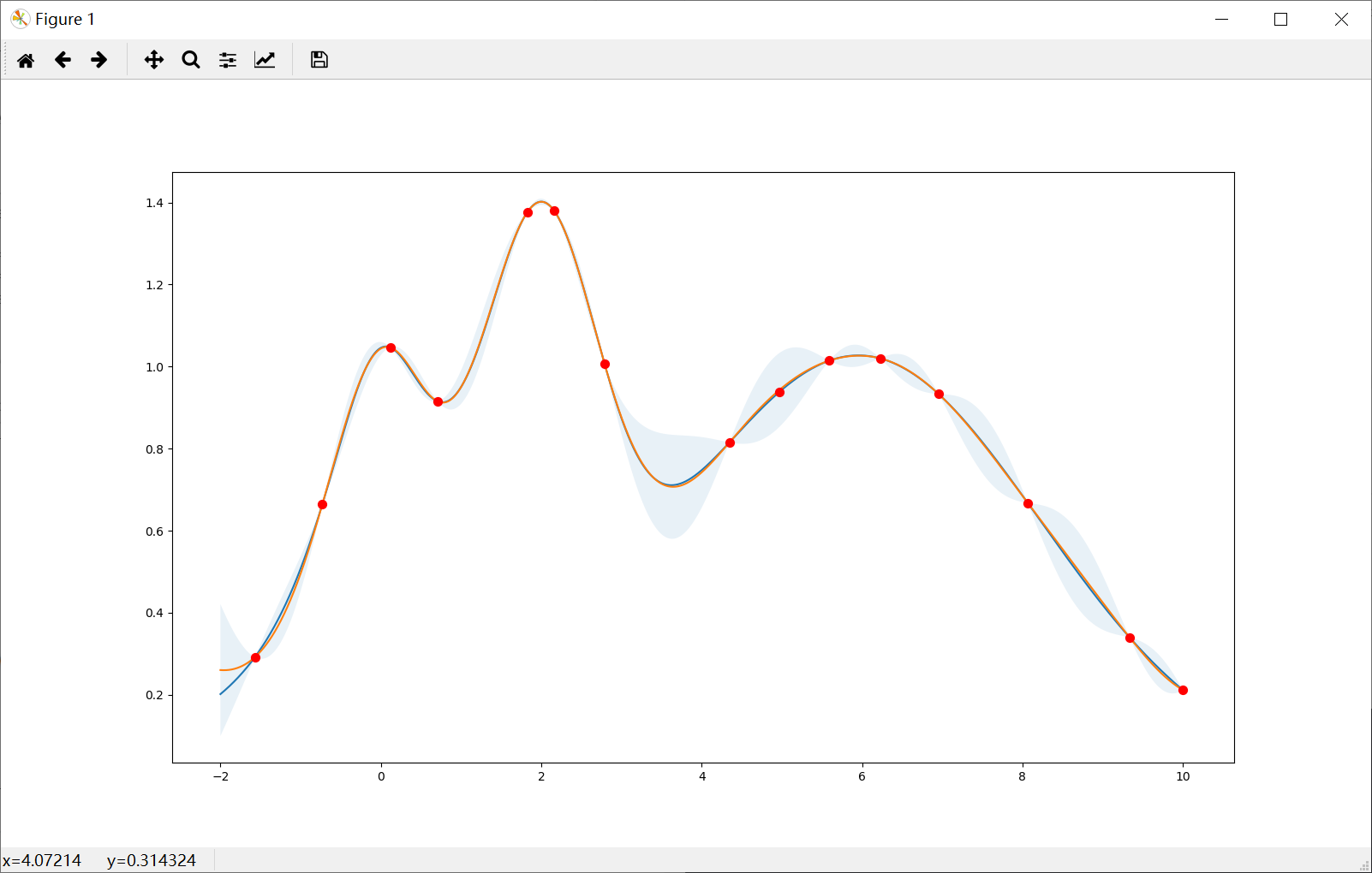
Prefer exploration (xi=1e-1)
Note that the points are more spread out across the whole range.
1 | bo = BayesianOptimization( |
Code
1 | import numpy as np |
Sequential Domain Reduction
Background
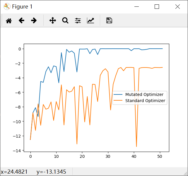
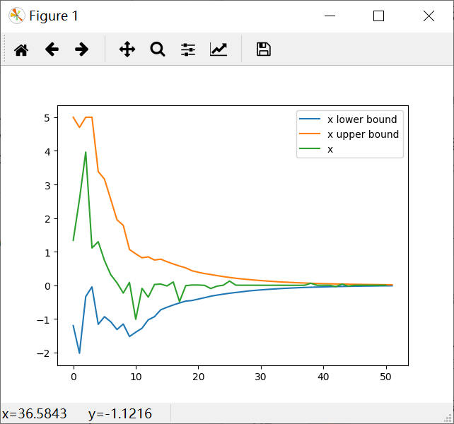
Sequential domain reduction is a process where the bounds of the optimization problem are mutated (typically contracted) to reduce the time required to converge to an optimal value. The advantage of this method is typically seen when a cost function is particularly expensive to calculate, or if the optimization routine oscilates heavily.
Basics
The basic steps are a pan and a zoom. These two steps are applied at one time, therefore updating the problem search space evey iteration.
Pan: recentering the region of interest around the most optimal point found.
Zoom: contract the region of interest.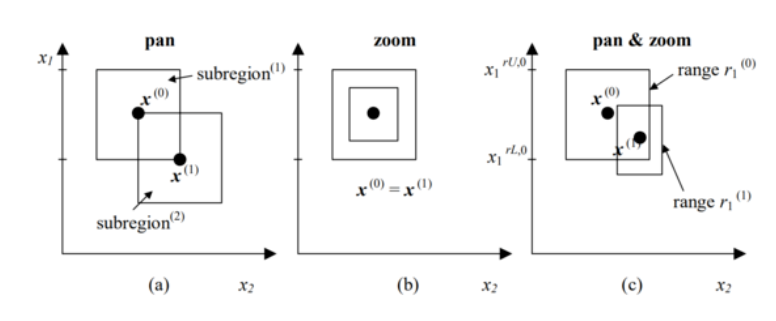
Parameters
There are three parameters for the built-in SequentialDomainReductionTransformer object:
$\gamma_{osc}:$ shrinkage parameter for oscillation. Typically [0.5-0.7]. Default = 0.7
$\gamma_{pan}:$ panning parameter. Typically 1.0. Default = 1.0
$\eta:$ zoom parameter. Default = 0.9
1 | import numpy as np |
Ideas for distributed fshion
1 | import time |
1 | optimizer 2 wants to register: {}. |
Deep Learning Example
1 | from mxnet import autograd, gluon, init, nd |
